
Zillow is one of the most successful real estate companies since the rise of the internet. Housing data is Zillow’s secret sauce and has enabled the use of tools like the Zillow Zestimate. Homebuyers, sellers, and real estate agents take advantage of the Zillow Zestimate as a rough means of estimating the value of a home. This tool is critical to the real estate industry, so why not figure out how they do it?
In this article, we will explore what it takes to build the Zillow Zestimate.

Agenda:
Gathering Data and Preprocessing
Machine Learning
Analyzing Estimator Input Features
Gathering Data and Preprocessing
Most real estate data is publicly accessible to those willing to find it. However, many of the companies that gather it in an easy-to-digest format restrict access to researchers like ourselves. So, to gather data to make a home value estimator like the Zestimate you have three options: Find online datasets (e.g. datasets), Buy the data (e.g. datarade), or Scrape your own data.
I chose the third option and built a real estate scraper that gathers sold house listing information from the Zillow website (more on this in a later article).
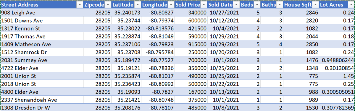
After scraping the data, I made a csv file of 1000 sold listings from 28205 in Charlotte, NC (note 1501 Downs Ave.):
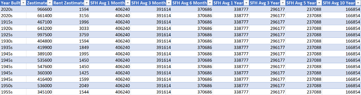
In addition to these features, I included information about the average market home value for single-family homes (SFHs) leading up to the sell date for each zip code (Zillow research). Also included was the year built, current home-value Zestimate, and rent Zestimate:
For preprocessing, features such as ‘Year Built’ and ‘Sold Date’ must be encoded to be properly used for machine learning purposes. Other categorical data attributes like ‘Street Address’ and ‘Zipcode’ must be dropped for many machine learning algorithms.
Machine Learning
The machine learning presented in this work uses python, scikit-learn, seaborn, and pandas. Each data column from our table represents a data feature. The goal will be to use a set of data columns x to map to a home value y using linear regression.
In addition to the preprocessing previously mentioned, I had to drop the ‘Zestimate’ and ‘Rent Zestimate’ data columns.
Final x columns: ‘Latitude’, ‘Longitude’, ‘Sold Date’, ‘Beds’, ‘Baths’, ‘House Sqft’, ‘Lot Acres’, ‘Year Built’, and the SFH average home value records.
Final y column: ‘Sold Price’
There are a few parameters to keep in mind. I sorted the data by date and used a 95% train, 5% test split on 1000 sold listings. Remember that split is used because we are using past listings to predict future ones with a home value estimate. It would not make sense to be training on housing data only from 2019 to predict housing prices from 2020 onwards, so this is a reasonable split. I also used StandardScaler() from scikit-learn to scale the data for the linear regression model as a last preprocessing step. Scaling the data is fundamental to a linear regression model. See more on this here.
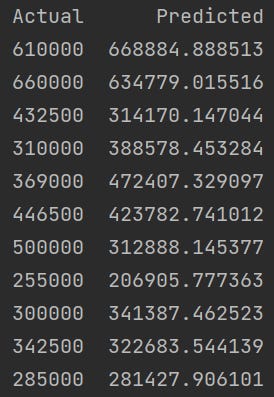
It is now time to fit our data and compare it to Zillow Zestimate. According to Zillow, the Zillow Zestimate has a 1.8% median error rate for active listings in the state of North Carolina. In other words, Zillow is very accurate. Our linear regression model has a median error rate of 18.6%. This may sound bad, but outliers skew the error. See predictions from our model below.
Clearly, this is not nearly as accurate as Zillow. Zillow likely uses more complex machine learning models than linear regression, uses more housing listings, and many more input features (e.g. ‘Has Water View’ or ‘Crime Rate’). The next section will look into how using different input features affect our results.
Analyzing Estimator Input Features
This section will analyze the input features that influenced the linear regression model performance. First, we will look at a correlation matrix to see the redundant input features. Second, we will examine the weight coefficients of our linear regression model to determine the most influential input features.
Correlation Matrix:
The correlation matrix displayed below highlights the redundant features in our linear regression model. Dark blue indicates a large positive correlation while bright yellow indicates a large negative correlation. Any two features with a correlation close to one, positive or negative, give our linear regression model similar (or redundant) information. Any two features with a correlation close to zero, indicated by light blue, bring unique information to our model.
For example, it makes sense below that latitude and longitude have a low degree of correlation, -0.3. The latitude of a house tells you nothing about the longitude of a house. However, beds and baths have a high degree of correlation, 0.69, because a large house with many beds likely has many baths as well.
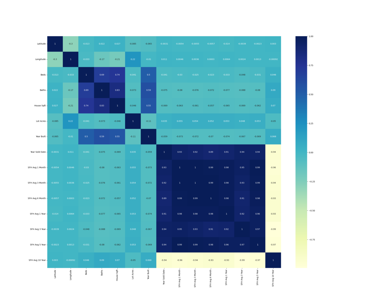
We learn a couple of things about our data from this correlation matrix. The first is that our ‘SFH Avg’ value over time features are redundant due to their high degree of correlation with each other, 0.89 to 1.0. If the ‘SFH Avg’ in the 28205 zip code is very low 1 month ago, it will likely be very low 3 months ago as well. This would be an area we can trim the fat in our model and drop some input features. The second is that the features ‘Lot Acres’ and ‘Year Built’ offer unique information to our linear regression model. Their low correlation value with all other features, less than 0.59, indicates these are unique features.
Linear Regression Weight Coefficients:
The correlation matrix is useful in showing us the unique and redundant features in our model, but it does not directly show us which features are most influential towards our outcome. For this, we must look at the weight coefficients.
As a quick example of a weight coefficient, say we had a linear regression model that only used beds and baths as input features. We then have a 3-bed 2-bath house that cost $350k. A pair of weight coefficients (excluding bias) would be a for bed and b for bath below:
350000 = a * 3 + b * 2
The weight coefficients a and b can be several different values. If a were 100,000 and b were 25,000, we would say beds are a more influential feature. If a were 50,000 and b were 100,000, we would say baths are a more influential feature. So what weight coefficients are largest for our home value linear regression model?
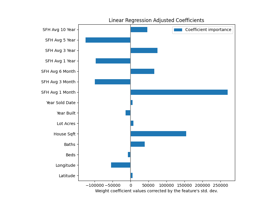
Ranking the coefficients suggest a couple of things about our input features. It is clear from the above figure that the most influential feature in home value is the average price of a home in the same zip code the previous month, aka ‘SFH Avg 1 Month’. The second most influential feature is ‘House Sqft’. These findings make sense to what we know about the housing market.
Something more interesting is that the longitude, or how East/West a house is, is a strong indicator of home value. The 28205 zip code lies to the East of downtown Charlotte, which suggests home values change with their longitude relative to downtown.
A final takeaway that may help improve our model is that SFH value averages make a significant impact on our model despite being largely redundant. It may be worth removing some of these features in later iterations to examine how it influences model quality.
Conclusion
This article taught us how to create a basic home value estimator, similar to the Zillow Zestimate, using linear regression. Although we can not match the Zillow Zestimate’s accuracy, we learned the tools necessary to build and improve our model with additional input features. These same building blocks can be extended to tools like home investment recommenders, which I will explore in a later article.
Thanks for reading and please comment with any questions or recommendations for future work!
Useful links: Coefficient interpretation ; Correlation Matrix w/ PCA